How To Create Excel Pie Chart

What is a Pie Chart and Why Use it?

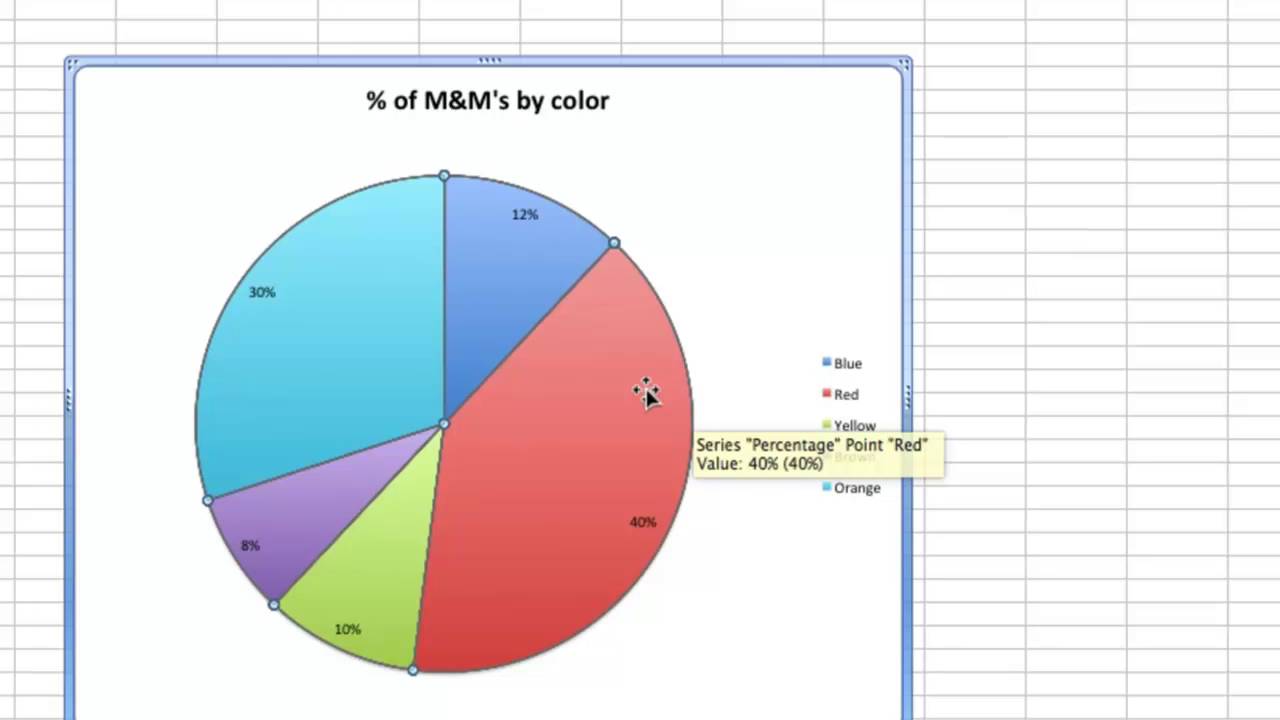
Excel pie charts are a great way to visualize data and show how different categories contribute to a whole. They are commonly used in business and academic settings to display survey results, sales data, and other types of information. In this article, we will walk you through the steps to create a pie chart in Excel, and provide tips on how to customize it to suit your needs.

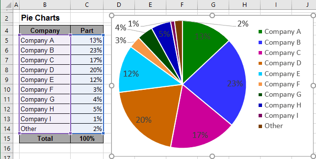
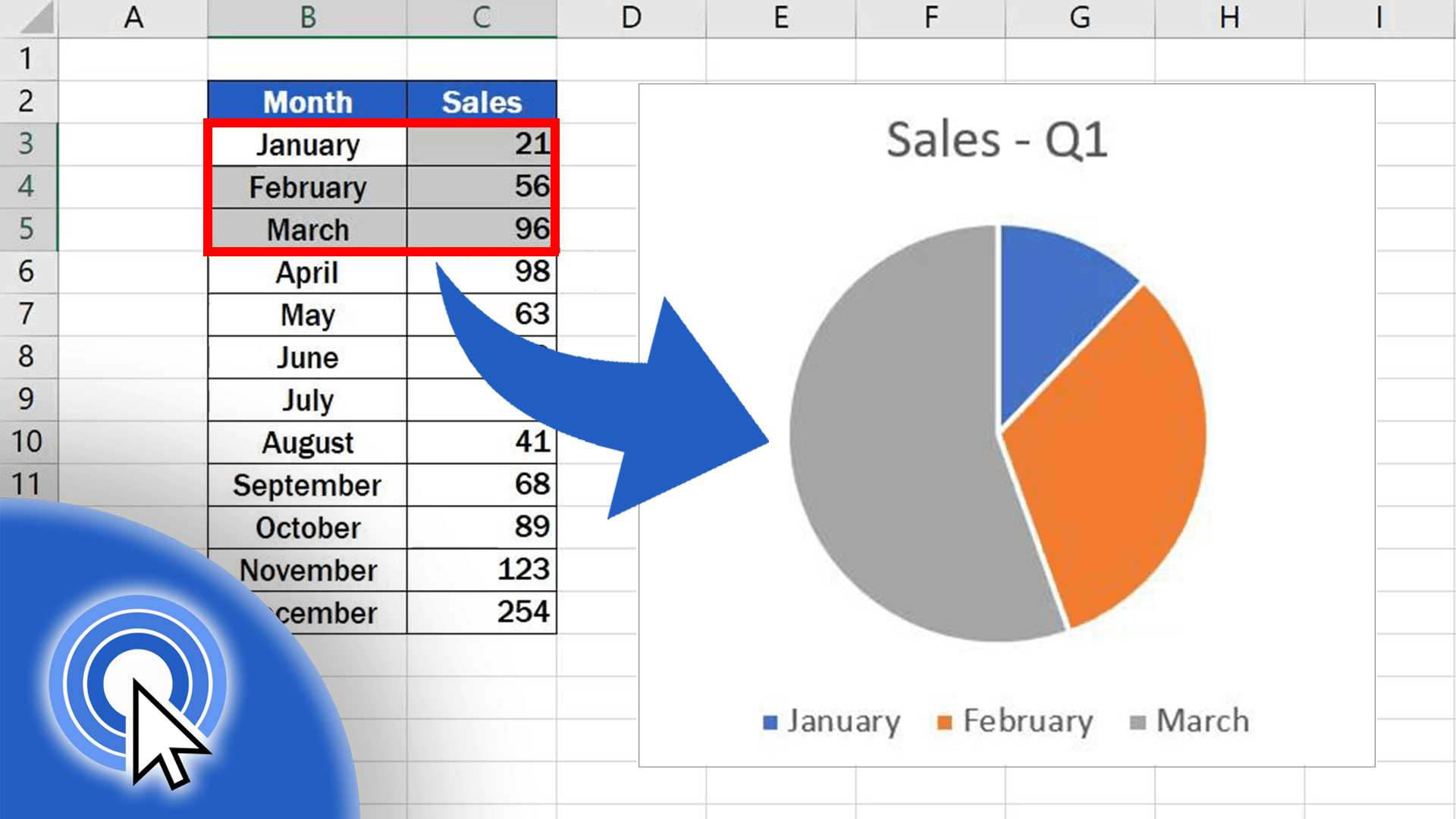
To create a pie chart in Excel, you will need to start by selecting the data you want to use. This should include the category names and the corresponding values. Once you have selected your data, go to the 'Insert' tab and click on the 'Pie' button in the 'Charts' group. This will open up a range of pie chart options, including 2D and 3D charts. Choose the type of chart you want to create and click 'OK' to insert it into your spreadsheet.

Customizing Your Excel Pie Chart

What is a Pie Chart and Why Use it? A pie chart is a circular chart that shows how different categories contribute to a whole. It is a great way to display data that adds up to 100%, such as survey results or sales data. Pie charts are easy to read and understand, making them a popular choice for presentations and reports. They can also be used to compare data across different categories, making it easy to see which categories are performing well and which ones need improvement.

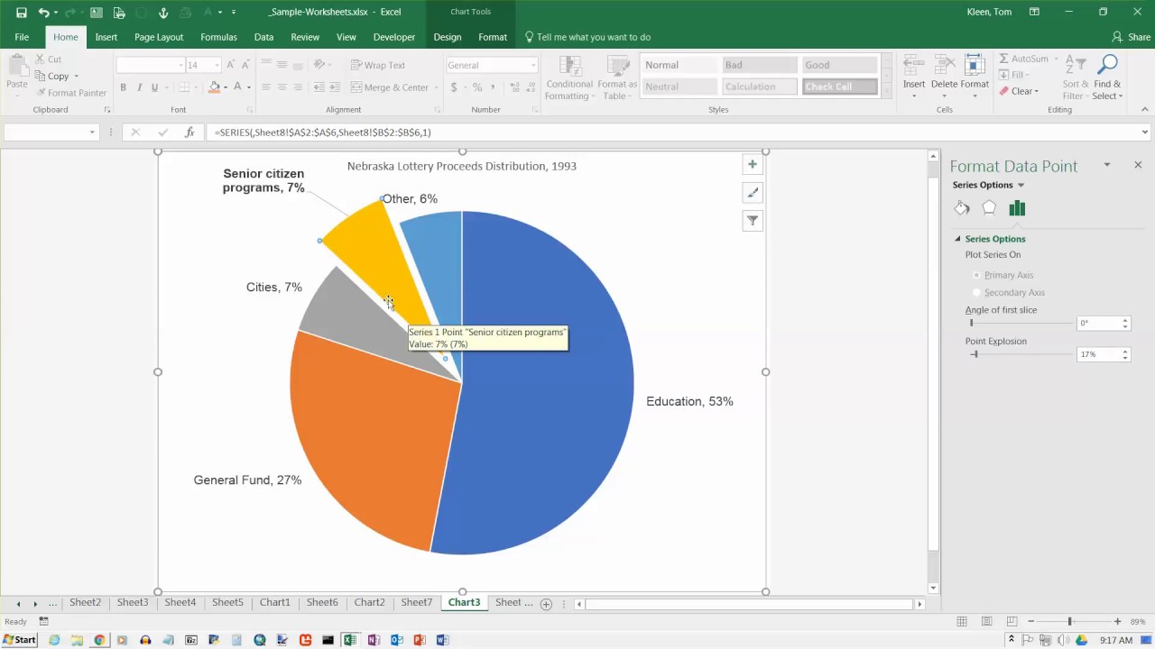
Customizing Your Excel Pie Chart Once you have created your pie chart, you can customize it to suit your needs. You can change the colors, add data labels, and adjust the chart title. You can also use the 'Chart Tools' tab to add additional features, such as a legend or axis labels. By customizing your pie chart, you can make it more visually appealing and easier to understand. With these steps, you can create a professional-looking pie chart in Excel that will help you to effectively communicate your data to others.